Statistical inference - Geophysical Data Analysis Book

Learning Objectives:¶

Distinguish the difference between probability and statistics.
Know what are population, parameter, sample, and statistic.
Build intuition for the Law of Large Numbers (LLN) and the Central Limit Theorem (CLT).
Explain why sample means fluctuate on the order of $1/\sqrt{n}$ and become more stable as sample size grows.
Know the estimator for variance.
Interpret a confidence interval correctly and connect its width to sample size.
Define null and alternative hypotheses and interpret the logic of a statistical test.

What is statistics and how is it different from probability?¶

Statistics and probability are closely related but address different directions of inference. Probability starts with a model of how outcomes are generated and asks what is likely to happen? It moves from known parameters to predictions about data. Statistics does the reverse: it starts with observed data and asks what can we infer about the underlying process?—it moves from data to unknown parameters. In short, probability is model → data, while statistics is data → model, and together they form the foundation for reasoning under uncertainty.

An example of flipping a Bernoulli coin¶

Suppose we are studying the process of flipping an uneven coin, following a Bernoulli random variable:

X \sim \mathrm{Bernoulli}(p)

(1)

where $p$ is the probability of success. Our goal is to infer the unknown $p$ using observed data: the head or tails of the coin flips.

Key definitions¶

Population¶

The population is the full conceptual collection of all possible outcomes generated by the process we are studying. Here, the population consists of infinitely many hypothetical Bernoulli trials:

X_1, X_2, X_3, \ldots \sim \text{i.i.d. Bernoulli}(p)

(2)

We never observe the full population; it is a theoretical object that defines the data-generating mechanism.

Parameter¶

A parameter is a fixed but unknown number describing the population. In this example, the parameter is:

p = \mathbb{P}(X = 1)

(3)

It controls the entire distribution and is the quantity of scientific interest.

Sample¶

A sample is a finite collection of observations drawn from the population. Suppose we observe $n$ independent Bernoulli trials:

x_1, x_2, \ldots, x_n

(4)

These are data, actual measurements.

Statistic¶

A statistic is any function of the sample (and only the sample). A natural statistic for estimating $p$ is the sample mean:

\hat{p} = \frac{1}{n}\sum_{i=1}^{n} x_i

(5)

This statistic is the empirical proportion of successes.

Let’s try this with code¶

In the next two Python cells, we simulate repeated flips of an uneven coin with true probability of heads $p = 0.6$ . Each flip is recorded as either 1 (success) or 0 (failure), so every trial is a Bernoulli random variable.

The experiment does three things:

It generates many independent sequences of coin flips.
It computes the running sample mean for each $n$
$\overline{X}_n = \frac{1}{n}\sum_{i=1}^{n} X_i,$
(6)
It compares those simulated sample means with the theoretical Law of Large Numbers scaling
$\mathrm{Std}(\overline{X}_n) = \frac{\sigma}{\sqrt{n}},$
(7)
where for a Bernoulli random variable,
$\sigma = \sqrt{p(1-p)}.$
(8)

In the figure, the faint green curves are many repeated experiments, the blue curve is one highlighted experiment, and the black lines show the true mean $p$ together with the expected $1/\sqrt{n}$ spread. As $n$ increases, the sample means cluster more tightly around the true mean.

import numpy as np
import matplotlib.pyplot as plt

# True Bernoulli parameter (population mean)
p_true = 0.6

# N flips in one experiment (for a concrete sample mean estimate)
N = 200

# Ensemble settings for LLN demonstration
N_max = 5000
n_ensemble = 1000

# No seed: each run will generate a different random sample
rng = np.random.default_rng()
# Binomial is a fast way to compute many Bernoulli trials at once: sum of 1's in n flips
flips = rng.binomial(1, p_true, size=(n_ensemble, N_max))

# Sample mean from one experiment with N flips
x_sample = flips[0, :N]
sample_mean_N = x_sample.mean()

# Running sample mean for each experiment: m_n = (1/n) * sum_{i=1}^n X_i
n_vals = np.arange(1, N_max + 1)
running_mean = np.cumsum(flips, axis=1) / n_vals

# Theoretical LLN spread for Bernoulli sample means
sigma = np.sqrt(p_true * (1 - p_true))
theory_std = sigma / np.sqrt(n_vals)
upper_band = p_true + theory_std
lower_band = p_true - theory_std

fig, ax = plt.subplots(figsize=(6, 4))

# Thirty sample-mean trajectories from repeated experiments
for k in range(20):
    ax.scatter(n_vals, running_mean[k], 0.05,marker='.', color="tab:green")
ax.scatter(n_vals, running_mean[k], 0.05,marker='.', color="tab:green", label="Monte Carlo trials")

# Theoretical mean and LLN spread
ax.axhline(p_true, color="black", ls="--", lw=2, label="True mean $p$")
ax.plot(n_vals, upper_band, color="black", lw=1.5, label=r"$p + \sigma/\sqrt{n}$")
ax.plot(n_vals, lower_band, color="black", lw=1.5, label=r"$p - \sigma/\sqrt{n}$")

ax.set_title("Bernoulli Coin Flips: Sample Mean Convergence")
ax.set_xlabel("Number of flips n")
ax.set_ylabel(r"$\overline{X}_n$")
ax.set_xlim(1, N_max)
ax.set_ylim(0.4, 0.8)
ax.legend()
fig.tight_layout()
plt.show()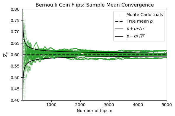

This $1/\sqrt{n}$ convergence rate is predicted by the Law of Large Numbers (LLN).

Limit Theorems¶

Law of Large Numbers (LLN)¶

Statement (informal)¶

Let $X_1, X_2, \dots$ be independent and identically distributed (i.i.d.) random variables with

\mathbb{E}[X_i] = \mu, \qquad \mathrm{Var}(X_i)=\sigma^2<\infty.

(9)

Define the sample average

\overline{X}_n = \frac{1}{n}\sum_{i=1}^n X_i.

(10)

As $n\to\infty$ ,

\overline{X}_n \to \mu \quad \text{with high probability}.

(11)

and

\mathrm{Var}(\overline{X}_N) = \mathrm{Var}\!\left(\frac{1}{N}\sum_{i=1}^N X_i\right) = \frac{1}{N^2}\sum_{i=1}^N \mathrm{Var}(X_i) = \frac{\sigma^2}{N}.

(12)

Intuition¶

When averaging many independent measurements, random fluctuations “cancel out.”
The average stabilizes around the true mean.
The distance from the true mean (the standard deviation) scales as $1/\sqrt{N}$ .
In geophysics: stacking traces reduces noise because signal adds coherently, noise adds incoherently.

Central Limit Theorem (CLT)¶

The Law of Large Numbers tells us that $\overline{X}_n$ gets close to $p$ . The Central Limit Theorem goes further: it tells us the shape of the fluctuations around $p$ .

Statement (informal)¶

Let $X_1,\dots,X_n$ be i.i.d. with mean $\mu$ and variance $\sigma^2$ .

The normalized sum

Z_n= \frac{\sum_{i=1}^n X_i - n\mu}{\sigma\sqrt{n}}

(13)

approaches a standard normal distribution as $n\to\infty$ :

Z_n \Rightarrow \mathcal{N}(0,1).

(14)

Intuition¶

Many small independent effects aggregate to produce a Gaussian shape.
Even if the underlying distribution is not Gaussian, the sum behaves Gaussian.
Explains why normal noise models are widely applicable.

# CLT experiment: distribution of Bernoulli sample means and standardized sums

n_trials = 50000
n_values_clt = [20, 100, 500]
bins_n = 20

x_grid = np.linspace(-4, 4, 400)
normal_pdf = np.exp(-0.5 * x_grid**2) / np.sqrt(2 * np.pi)

# Simulate once per n, then reuse the same draws for both panels
sample_mean_by_n = {}
z_by_n = {}
for n in n_values_clt:
    samples = rng.binomial(1, p_true, size=(n_trials, n))
    sample_mean_by_n[n] = samples.mean(axis=1)
    z_by_n[n] = (samples.sum(axis=1) - n * p_true) / (sigma * np.sqrt(n))

fig, (ax_left, ax_right) = plt.subplots(1, 2, figsize=(8, 4))
colors = {20: "tab:blue", 100: "tab:orange", 500: "tab:green"}

# Left panel: distribution of sample mean for increasing n
mean_grid = np.linspace(
    p_true - 4 * sigma / np.sqrt(min(n_values_clt)),
    p_true + 4 * sigma / np.sqrt(min(n_values_clt)),
    400,
 )

for n in n_values_clt:
    sample_means = sample_mean_by_n[n]
    approx_sd = sigma / np.sqrt(n)
    normal_mean_pdf = np.exp(-0.5 * ((mean_grid - p_true) / approx_sd) ** 2) / (approx_sd * np.sqrt(2 * np.pi))

    ax_left.hist(
        sample_means,
        bins=bins_n,
        density=True,
        alpha=0.25,
        color=colors[n],
        edgecolor="white",
        linewidth=0.5,
        label=fr"n={n}",
    )
    ax_left.plot(
        mean_grid,
        normal_mean_pdf,
        color=colors[n],
        lw=2,
    )

ax_left.set_title("Histogram and CLT Gaussian Sample Mean")
ax_left.set_xlabel(r"$\overline{X}_n$")
ax_left.set_ylabel("Density")
# ax_left.set_xlim(0.2, 1)
# ax_left.set_ylim(0, 30)
ax_left.legend(fontsize=8)

# Right panel: standardized sample mean approaches N(0,1)
for n in n_values_clt:
    ax_right.hist(
        z_by_n[n],
        bins=bins_n,
        density=True,
        histtype="step",
        color=colors[n],
        lw=2.2,
        label=fr"n={n}",
    )

ax_right.plot(x_grid, normal_pdf, color="black", lw=2.5, label=r"$\mathcal{N}(0,1)$")
ax_right.set_title("Standardized Bernoulli Sums Histograms")
ax_right.set_xlabel(r"$Z_n$")
ax_right.set_ylabel("Density")
ax_right.set_xlim(-4, 4)
ax_right.legend(fontsize=8)

fig.suptitle("Central Limit Theorem for Bernoulli Random Variables", fontsize=12)
fig.tight_layout()
plt.show()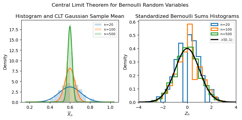

Estimating Variance¶

Let $X_1, \dots, X_n$ be i.i.d. samples from a distribution with mean $\mu$ and variance $\sigma^2$ .

We have the sample mean

\bar{X} = \frac{1}{n}\sum_{i=1}^n X_i

(15)

The naive variance estimator¶

The naive estimator divides by $n$ :

s_n^2 = \frac{1}{n}\sum_{i=1}^n (X_i - \bar{X})^2

(16)

This estimator is biased, meaning

\mathbb{E}[s_n^2] = \frac{n-1}{n}\sigma^2

(17)

It systematically underestimates the true variance.

Unbiased Variance Estimator (Bessel’s Correction)¶

To remove the bias, divide by $n - 1$ :

s^2 = \frac{1}{n-1}\sum_{i=1}^n (X_i - \bar{X})^2

(18)

Then

\mathbb{E}[s^2] = \sigma^2

(19)

so this estimator is unbiased.

Intuition: Estimating the mean $\bar{X}$ from the same data uses up one degree of freedom. Thus, dividing by $n-1$ compensates for the fact that the residuals $(X_i - \bar{X})$ are constrained to sum to zero.

Remarks¶

The Bessel’s correction has a smaller effects for larger $n$ . Therefore, for large amount of data, either formula can be used.

Note, the numpy numpy.var function defaults to the bias estimator. You can read about it here.

Confidence Intervals¶

Definition¶

Let $\theta$ be an unknown population parameter and $\hat{\theta}$ an estimator based on a sample of size $n$ . A $(1-\alpha)\times 100\%$ confidence interval is a random interval $[L,\, U]$ — computed from the data — that satisfies

\mathbb{P}(L \le \theta \le U) = 1 - \alpha

(20)

For a 95% CI, $\alpha = 0.05$ .

The interval is random because $L$ and $U$ depend on the sample. The correct interpretation is: if we repeated the experiment many times, $(1-\alpha)$ of those intervals would contain the true $\theta$ . A single realized interval either covers $\theta$ or it does not.

General CLT-based interval¶

Whenever the CLT applies, we have an approximate $(1-\alpha)$ confidence interval for $\mu$ :

\bar{X}_n \pm z_{\alpha/2} \, \frac{\hat{\sigma}}{\sqrt{n}}

(21)

where $z_{\alpha/2}$ is the upper $\alpha/2$ quantile of the standard normal (e.g. $z_{0.025} = 1.96$ for 95% CI) and $\hat{\sigma}$ is an estimate of the population standard deviation.

The width of the interval shrinks like $1/\sqrt{n}$ , consistent with the LLN rate we saw earlier.

Illustration: Bernoulli coin-flip experiment¶

In the coin-flip example, we observe $n$ flips of a coin with unknown bias $p$ and estimate it with

\hat{p} = \frac{1}{n}\sum_{i=1}^n X_i

(22)

Since $\mathrm{Var}(X_i) = p(1-p)$ , the CLT-based standard error is

\mathrm{SE}(\hat{p}) = \sqrt{\frac{p(1-p)}{n}} \approx \sqrt{\frac{\hat{p}(1-\hat{p})}{n}}

(23)

and the 95% confidence interval is

\hat{p} \pm 1.96 \sqrt{\frac{\hat{p}(1-\hat{p})}{n}}

(24)

This is consistent with the $1/\sqrt{n}$ band we plotted in the LLN figure: the confidence interval is essentially one snapshot of that shrinking uncertainty band, evaluated at your observed $\hat{p}$ .

# Empirically test the 95% CLT confidence interval for a Bernoulli parameter

n_flips = 200          # sample size per experiment
n_experiments = 2000  # number of repeated experiments
z_95 = 1.96           # z-score for 95% CI

# Simulate many independent experiments, each with n_flips coin flips
all_flips = rng.binomial(1, p_true, size=(n_experiments, n_flips))

# Estimate p and the 95% CI for each experiment
p_hat = all_flips.mean(axis=1)
se = np.sqrt(p_hat * (1 - p_hat) / n_flips)
ci_lower = p_hat - z_95 * se
ci_upper = p_hat + z_95 * se

# Check which intervals actually contain the true p
contains = (ci_lower <= p_true) & (p_true <= ci_upper)
coverage = contains.mean()

# Plot the first 60 intervals, highlighting misses
n_show = 60
fig, ax = plt.subplots(figsize=(8, 4))

for i in range(n_show):
    color = "tab:blue" if contains[i] else "tab:red"
    ax.plot([ci_lower[i], ci_upper[i]], [i, i], color=color, lw=1.4, alpha=0.7)
    ax.plot(p_hat[i], i, "o", color=color, ms=3)

ax.axvline(p_true, color="black", lw=2, ls="--", label=f"True $p = {p_true}$")
ax.set_xlabel(r"$p$")
ax.set_ylabel("Experiment index")
ax.set_title(
    f"95% CIs for {n_show} experiments  "
    f"(blue = covers $p$, red = misses)\n"
    f"Empirical coverage: {coverage*100:.1f}% over {n_experiments} total experiments"
)
ax.legend()
fig.tight_layout()
plt.show()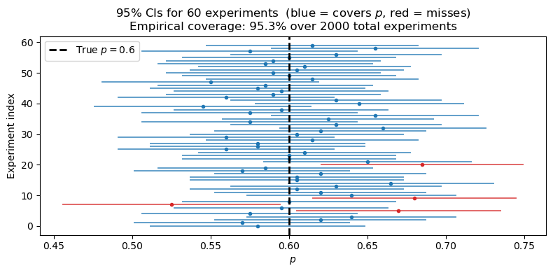

Null Hypothesis and Statistical Testing¶

So far, we have focused on estimation: using data to estimate an unknown parameter such as $p$ or $\mu$ . Often, however, the goal is to evaluate a specific claim about that parameter.

Null and alternative hypotheses¶

A null hypothesis $H_0$ is a baseline claim about the parameter. It usually represents a default position, such as “no effect,” “no difference,” or a specific reference value.

An alternative hypothesis $H_A$ is the competing claim we would support if the data look inconsistent with $H_0$ .

For the Bernoulli coin example, we might test whether the coin is fair:

H_0: p = 0.5 \qquad \text{versus} \qquad H_A: p \ne 0.5

(25)

Here, $H_0$ says the probability of heads is exactly 0.5, while $H_A$ says it is different from 0.5.

General idea of a statistical test¶

A statistical test asks: if the null hypothesis were true, would the statistic we observed be unusually far from what $H_0$ predicts?

The usual ingredients are:

A null hypothesis $H_0$ and an alternative hypothesis $H_A$ .
A test statistic computed from the sample.
A reference distribution for that statistic assuming $H_0$ is true.
A rule for deciding whether the observed result is surprising enough to reject $H_0$ .

Bernoulli example with the CLT¶

If $X_1, \dots, X_n \sim \mathrm{Bernoulli}(p)$ , then the sample proportion is

\hat{p} = \frac{1}{n}\sum_{i=1}^n X_i

(26)

Under the null hypothesis $H_0: p = p_0$ , the CLT tells us that for large $n$ ,

\hat{p} \approx \mathcal{N}\!\left(p_0,\, \frac{p_0(1-p_0)}{n}\right)

(27)

so the standardized test statistic is approximately

Z = \frac{\hat{p} - p_0}{\sqrt{p_0(1-p_0)/n}} \approx \mathcal{N}(0,1)

(28)

If $|Z|$ is large, then the observed $\hat{p}$ is far from what we would expect if $H_0$ were true, which is evidence against the null hypothesis.

p-value and significance level¶

The p-value is the probability, assuming $H_0$ is true, of obtaining a result at least as extreme as the one observed.

A small p-value means the data would be unusual under the null model. A common threshold is $\alpha = 0.05$ :

If the p-value is less than $\alpha$ , we reject $H_0$ .
If the p-value is greater than or equal to $\alpha$ , we fail to reject $H_0$ .

Failing to reject $H_0$ does not prove that $H_0$ is true. It only means the data do not provide strong enough evidence against it.

Connection to confidence intervals¶

For a two-sided test, there is a direct link to the confidence intervals we already introduced: a level- $\alpha$ test rejects $H_0: \theta = \theta_0$ exactly when $\theta_0$ falls outside the $(1-\alpha)$ confidence interval for $\theta$ .

So confidence intervals and hypothesis tests are two ways of expressing the same inferential uncertainty.

Important interpretation¶

A hypothesis test is a decision rule with long-run error properties. It does not tell us the probability that the null hypothesis is true, and statistical significance does not automatically imply scientific or practical importance.

Key Points¶

Statistical inference uses observed data to learn about unknown features of a population or data-generating process.
A parameter is an unknown quantity that describes a population, a sample is a finite set of observations, and a statistic is a quantity computed from that sample to estimate the parameter.
The Law of Large Numbers says that the sample mean approaches the true mean as the sample size increases.
The variability of the sample mean scales like $1/\sqrt{n}$ , so larger samples produce more stable estimates.
The Central Limit Theorem says that properly standardized sums or sample means become approximately Gaussian for large $n$ , even when the original data are not Gaussian.
The variance estimator that divides by $n$ is biased low; dividing by $n-1$ gives an unbiased estimator.
A confidence interval is a procedure that captures the true parameter with a stated long-run frequency, not a probability statement about a single fixed parameter after the data are observed.
A null hypothesis is a baseline claim about a parameter, and a statistical test checks whether the observed data would be unusually inconsistent with that claim.
A p-value measures how surprising the observed result would be if the null hypothesis were true.
Confidence intervals and two-sided hypothesis tests are closely connected: a null value is rejected at level $\alpha$ when it lies outside the corresponding $(1-\alpha)$ confidence interval.
Confidence interval width shrinks as sample size increases.